Lecture 12: Projective Structures on Surfaces Part II

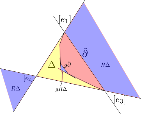
Last time we introduced properly convex projective structures on surfaces with principal totally geodesic boundary. We proved a few basic lemmas about how \(\Omega\) was situated in \(\mathbb{R}P^2\), when \(\Omega/\Gamma\) is a projective manifold with principal totally geodesic boundary. The figure below illustrates the generic configuration.

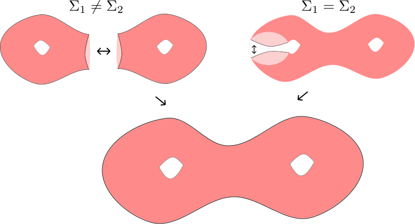
We now discuss how we can glue properly convex surfaces with principal boundary to get new properly convex surfaces. Here is the setup: Let \(\Sigma_1=\Omega_1/\Gamma_1\) and \(\Sigma_2=\Omega_2/\Gamma_2\) be properly convex surfaces (here it is possible that \(\Sigma_1=\Sigma_2\)) with principal boundary components \(\partial_1\) and \(\partial_2\). Let \(f:N(\partial_2)\to N(\partial_2)\) be a projective equivalence between principal annular neighborhoods of \(\partial_1\) and \(\partial_2\). Using this projective equivalence we can produce a (non-unique) projective structure on the manifold \(\Sigma:=\Sigma_1\sqcup_f \Sigma_2\), such that the obvious inclusion maps \(\iota_i:\Sigma_i\to \Sigma\) for \(i=1,2\) are projective embeddings. Two possibilities can arise depending on whether or not \(\Sigma_1=\Sigma_2\) (see figure below).

Theorem: Let \(\Sigma_1\) and \(\Sigma_2\) be as above then the projective structure on \(\Sigma\) is properly convex. In other words \(\Sigma\cong \Omega/\Gamma\), for some properly convex \(\Omega\) and some discrete group \(\Gamma\subset PGL(\Omega)\).

We will focus on the case where \(\Sigma_1\neq \Sigma_2\), as the proof in the other case requires only small modifications.

We begin by describing both the holonomy and developing map of this structure. Let \(\Gamma=\pi_1\Sigma\), let \(\partial\) be the image of \(\partial_1\) in \(\Sigma\) and let \(\gamma\) be such that \(\langle\gamma\rangle=\pi_1\partial\). By Van Kampen we see that \(\Gamma\cong \Gamma_1\ast_{\pi_1\partial} \Gamma_2\). For \(i=1,2\) let \(\rho_i:\pi_1\Sigma_i\to \Gamma_i\) be the holonomy of the projective structure on \(\Sigma_i\) and assume we have conjugated so that \(\rho_1(\pi_1\partial_1)=\rho_2(\pi_1\partial_2)\). Let \(g\in \Gamma\) then we can write \(g=\gamma_1\gamma_2\cdots \gamma_m\) where \(\gamma_i\in \Gamma_{i \text{ mod } 2}\). We can define the holonomy representation \(\sigma:\pi_1\Sigma\to SL_3(\mathbb{R})\) as

Note that this is well defined since we insisted that \(\rho_1(\pi_1\partial_1)=\rho_2(\pi_1\partial_2)\). In order to define the developing map we need to give a “combinatorial description” of \(\tilde \Sigma\). Informally, the universal cover can be described as follows. Pick a lift of \(\tilde \Sigma_1\) to \(\tilde \Sigma\). This lift will contain infinitely many copies of \(\tilde \partial\) (one for each \(\Gamma_1\) conjugate of \(\pi_1\partial\)). Along each of these copies of \(\tilde \partial\) we glue a copy of \(\tilde \Sigma_2\). Each of the copies of \(\tilde \Sigma_2\) that we have glued on will itself contain infinitely many copies of \(\tilde \partial\). Along each of these we glue a copy of \(\tilde \Sigma_1\). Repeating this procedure ad infinitum gives a tiling of \(\tilde \Sigma\) where the tiles are copies of \(\tilde \Sigma_1\) and \(\tilde \Sigma_2\) glued along \(\tilde \partial\).

More formally, For \(i=1,2\), let \(\hat T_i=\Gamma\times \Omega_i\). There is a group action of \(\Gamma_i\) on \(\hat T_i\) given by \(\alpha\cdot(\gamma,p)=(\gamma\alpha^{-1}),\alpha\cdot p)\). If we let \(T_i=\hat T_i/\Gamma_i\) then \(\tilde \Sigma=T_1\sqcup T_2\) where we identify the points \([(\gamma,p)]\in T_1\) and \([(\gamma,p)]\in T_2\) whenever \(p\in \Omega_1\cap \Omega_2\). Sets fo the form \(\{\gamma\}\times \Omega_i\) are called tiles can be thought of as the aforementioned copies of \(\tilde \Sigma_i\) that tile \(\tilde \Sigma\). The action of \(\Gamma\) on \(\tilde \Sigma\) by deck transformations is given by \(g\cdot[(\gamma,p)]=[(g\gamma,p)]\)

Using this description it is a very simple matter to describe the developing map. If we let \([(\gamma,p)]\in \tilde \Sigma\) then

By construction, \(Dev\) is \(\sigma\)-equivariant.

In order to prove the above theorem we will show that \(Dev\) is an embedding onto a properly convex subset of \(\mathbb{R}P^2\). This will be done by applying a ping-pong arguement. The crux of this argument is the following fact that follows from the main lemma from the previous lecture. Let \(\gamma\) be such that \(\langle \gamma\rangle=\pi_1\partial\) then for any \(g\in \Gamma_1\setminus\langle\gamma\rangle\) \(g\Omega_2\subset \Delta\setminus \Omega_1\) and for any \(g\in \Gamma_2\setminus \langle \gamma\rangle\) \(g\Omega_1\subset R\Delta\setminus\Omega_2\).

We begin by showing that \(Dev\) is injective. To this end let \([(\gamma_1,p_1)]\) and \([(\gamma_2,p_2)]\) be distinct points in \(\tilde \Sigma\). By renumbering we can assume that \(p_2\in \Omega_1\). Furthermore, by applying a deck transformation we can assume that \(\gamma_1=1\). By construction, the developing map restricted \(\Omega_1\cup\Omega_2\) is injective. It follows that the restriction of the developing map to any adjacent tiles is injective. As a result, we can assume that \(\gamma_2\notin \Gamma_1\cup\Gamma_2\). It thus suffices to show that \(\sigma(\gamma_2)\Omega_1\) is disjoint from \(\Omega_1\cup\Omega_2\). By our previous simplifications, we can assume that \(\gamma_2=g_1g_2\cdots g_m\), where \(g_i\in (\Gamma_1\cup\Gamma_2)\setminus \langle\gamma\rangle\) and \(g_i\in \Gamma_1\) if and only if \(g_{i+1}\in \Gamma_2\).

We can now play ping-pong. As usual, there are a few cases to consider. First, suppose that \(g_m\in \Gamma_2\). In this case

In the case where \(g_m\in \Gamma_1\) we simply observe that \(\Gamma_1\) preserves \(\Omega_1\) and then apply the above argument to \(g_1\cdots g_{m-1}\). As a result \(Dev\) is injective. Since developing maps are in general local embeddings we conclude that \(Dev\) is an embedding onto its image, which we now show is a convex set. The image of \(Dev\) can be constructed as an increasing union of tiles. It is easily verifed that the connected union on tiles has locally convex boundary and is thus convex. Therefore the image of \(Dev\) is an increasing union of convex sets and is thus convex. To see that the image is proper we observe that the above ping-pong argument actually shows that

and this last set is disjoing from any hyperplane passing through \([e_2]\) and disjoint from \(\Delta\cup R\Delta.\) This completes the proof of the theorem.

While the above theorem tells us that we can convexly glue properly convex surfaces along principal boundary components provided their boundary geometry matches, it does not tell us in how many ways this can be done. It turns out such a gluing can be done in 2 dimensions worth of ways. More concretely, since \(\pi_1\partial\) is conjugate into \(D^+\) we see that \(\pi_1\partial\) is centralized by a fixed conjugate of any element of \(D^+\). Given such a centralizing element \(\alpha\) we apply \(\alpha\) to \(\Omega_2\) in our construction of the developing map. Different choices of \(\alpha\) give rise distinct marked convex projective structures. Informally, the geometries of \(\Sigma_1\) and \(\Sigma_2\) are indepentent of \(\alpha\). What \(\alpha\) is affecting is the way that these structures are glued together.

In the next lecture we will conclude our discussion of convex projective structures on surfaces by describing the space of convex projective structrures with principal boundary on a pair of pants.

Previous Post: Lecture 11: Projective Structures on Surfaces

Next Post: Lecture 13: Projective Structures on Surfaces Part III